


“Green light, STOP – if you want to see where you are taking the most risk, look where you are making the most money.” – Paul Gibbons.
One of the most oft-quoted pearls of wisdom emanating from Investment analysts with regard to risk control is “Enjoy the party but dance near the door“. It has been said and written so often that it IS an investment cliche, but it is an inappropriate metaphor. After all, the worst that could happen is that you run out of drink (and being near the door is of no help in that regard). A more relevant comparison is with that of a homeowner, who lives on a tectonic fault line. One may decide that, as there hasn’t been a “Big One” since 1906 (and is, according to seismologists, now overdue) and if one were to feel a succession of small rumblings for a period of time, that it may be prudent to consider moving a little further away from the earthquake zone- not too far, however, as one still has to commute into work, but far enough away that a major “event” would not be catastrophic for ones finances (obviously, earthquake insurance is not covered in one’s Home Insurance Policy and is extremely expensive). This is how we see the current market situation; as we showed last week, there are some signs of “rumblings ” beneath the surface of the rapid price gains. It is important to control what you can and let markets do what they will. That control is in the area of risk.
So what does one do? Selling everything would be a huge bet on a market decline and is not a wise strategy- after all, the “Big One”- a market crash in this instance- may not hit for months or years (or even at all!). A sensible approach may be to lower market exposure, while maintaining a risk profile that allows for continued gains should a major fall not happen. Fortunately there are a couple of ways to look at this problem, both of which should allow investors to reap the benefits of investing in the major asset classes, while keeping market risk within tolerable levels. Given the mathematics of compound returns [1], it is important to ensure that a loss does not de-rail the investment target.
There are two ways to look at market risk; either via portfolio duration or portfolio volatility. Let us look at both of these in turn, using the MSCI World Index (as a proxy for the World Stock market and then EBI 100, EBI 70 and EBI 40 to illustrate the effect of lowering overall portfolio volatility.
Portfolio Duration:
We have covered this concept in previous blogs (see here). The idea of bond duration is reasonably well understood, but the concept of equity duration less so. As the post referred to says, equity duration can be approximated by the Price: Dividend ratio. So, for example, the MSCI World Index is currently at 2230 (as of 24/1/18) and yields around 2.2%. which equates to a duration of (2230/49.1 = 45.4 years) [2]. The Vanguard Total Bond Market ETF will be used as the Bond market surrogate, which has a Duration of 6.1 years at present.
It is a basic premise of investing that ones time horizon and portfolio duration should be aligned as closely as possible in order to reduce (or preferably eliminate) the risk of path dependency- that is, the risk that the investment return is not generated to match expectations until after the investor needs the money [3].
The conventional portfolio allocation is 60:40 stocks and bonds, which therefore has a duration of (0.6 x 45.4 + 0.4 x 6.1 = 29.68 years). This is thus not necessarily suitable for everyone. With UK Life expectancy currently just under 81 years (on average of course, which leaves a fair amount of room for discretion), it may be that many close to retirement might need to re-think their allocations in a downwards direction. Viewed in this light, 100% exposure to equities may only be appropriate for those in their 30’s. Using the same formula as above, a 40:60 portfolio, however, has a duration of just under 22, which may be far more closely aligned to actual investor time horizons. The possible permutations are of course almost endless.
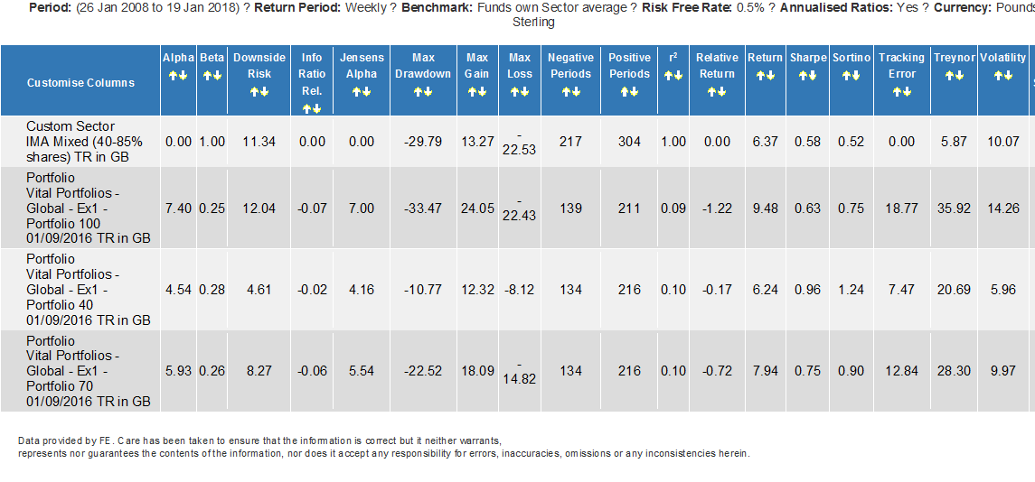
Now, let us look at the problem through the lens of portfolio (price) volatility. The chart below shows this phenomenon using 3 EBI portfolios. It is important to bear in mind that as a low cost provider the situation could be far worse in a more expensive (read: Active) portfolio. To the extent that the portfolio costs are higher than EBI, the scenarios painted could be best case ones.
Below we can see the returns and volatility numbers for the three portfolios (plus a Sector Index for context). Using a Standard Normal Distribution Table, we can estimate the probability (and extent) of a decline in prices by a set amount (in the jargon, a standard deviation event-SD). For example, a 2 SD event (which has a 2.28% probability of occurrence- or 1 week in 44) could lead to a decline of 19.04%, 12% and 5.68% for EBI 100, 70 and 40 respectively [4].
But in the market context, we must recognise that things could get far worse than a 2 SD decline (obviously, a 2 SD RISE of no concern). For anything greater than a 2 SD event, we need to recognise that extreme events occur more frequently than conventional statistics imply. For that, we need to use a Cubic Power Law, which better captures the reality that stock price moves are not normally distributed, (because Investors tend to panic at more or less the same time, resulting in major market moves “clustering” in short periods).
Using this formula [5] for 3 SD moves, one gets a better indication of how prices can move (and at what probability) in reality, rather than in an economist’s classroom.
Using the same calculation as in [4], a 3 Standard Deviation event would cause a decline of 33.3%, 21.97% and 11.64% for the respective (100, 70 and 40) portfolios. Clearly, this is not to say that these events WILL occur, but it gives an idea of the potential magnitude of the price declines should they do so. In the case of EBI 100, a 33% decline would require the portfolio to double to get back to “break-even”, (which has occurred post 2003 AND 2009), but the question then becomes, how quickly can markets recover; if the investor is close to retirement, there may not be enough time for that to happen. In the case of EBI 40, it would need only a 13.1% price gain to recover the previous level, which is a much easier task.
At present, it looks as if risk has been abolished, as Investors abandon hedges almost completely, but this will not last, (nothing does). By the time risk reduction is needed, it may be too late, as prices will have (possibly violently) adjusted. Paradoxically, the time to focus on risk control is precisely the time that no-one sees the need for it; it appears that we are approaching that point.
According to this article (quoting a Credit Suisse research note), US Pension funds may need (as part of their monthly re-balancing process) to sell up to $12 billion in equities (buying $24 billion in bonds) in the coming days. As they say in the best sci-fi films, maybe “we are not alone” in thinking this way.
[1] For example, assume 3 years of 10% annual portfolio growth, a £100,000 portfolio would, at the end of year 3, be worth £133,100. However, a 10% loss in year 4 leaves the Investor with just £119,790; in the process, the annualised return for the portfolio drops from 10% p.a. after year 3 to just 4.62% in year 4. (and a 20% loss leaves the annual return at a mere 1.58% p.a.) If the market were to rise another 10% in year 4, but then fall 10% in year 5 the annualised return would be 5.67% p.a.
On the other hand, if the portfolio is positioned such that it only falls 5% in both of the above examples, the 4-year return becomes 6.04% p.a. and 6.82% respectively. Risk control is very tolerant of positions taken, even those that are somewhat early in the piece…
[2] A quicker way to calculate this is to divide 100 by the dividend yield. The result is the same.
[3] To illustrate, assume £100 is invested for a time horizon of 30 years, with an expected return of 5% per annum. (£432.19 on retirement). If however, the portfolio duration is longer than 30 years, (e.g. 40 years), it is entirely possible that the same 30-year return could be achieved, but only after the investor has need of the cash (say, in years 35-40). This mismatch creates the risk that the investments will achieve the required rate of return in time for the investor to benefit from them, as there is guarantee of a simple 5% annual return every year. There will periods of losses, potentially in years 28-30.
[4] This is determined by multiplying the portfolio Volatility by 2 (to get the 2 SD amount) and taking this from the annualised return number. So, for EBI 100, the calculation is 9.48- (2 x 14.26) = -19.04% . Doing the same for the other two gives us a decline of 12% and 5.68%.
[5] To calculate this, we must ask how much less likely is a 3 SD move than a 2 SD event, where the latter has a 2.28% chance of occurring. We divide 3 by 2 (because we are only interested in the bad half of the distribution) and the raise it to the power of three (1.5^3). This (4.56) we then divide into 2.28 to get 0.5%. 100 divided by 0.5= 200 or one week in 200 (1 week in every 3.8 years).
Disclaimer
We do not accept any liability for any loss or damage which is incurred from you acting or not acting as a result of reading any of our publications. You acknowledge that you use the information we provide at your own risk.
Our publications do not offer investment advice and nothing in them should be construed as investment advice. Our publications provide information and education for financial advisers who have the relevant expertise to make investment decisions without advice and is not intended for individual investors.
The information we publish has been obtained from or is based on sources that we believe to be accurate and complete. Where the information consists of pricing or performance data, the data contained therein has been obtained from company reports, financial reporting services, periodicals, and other sources believed reliable. Although reasonable care has been taken, we cannot guarantee the accuracy or completeness of any information we publish. Any opinions that we publish may be wrong and may change at any time. You should always carry out your own independent verification of facts and data before making any investment decisions.
The price of shares and investments and the income derived from them can go down as well as up, and investors may not get back the amount they invested.
Past performance is not necessarily a guide to future performance.