[Note that this analysis will concentrate primarily on US Indices, as there is more available data, but it will inevitably apply to other markets as they tend to mimic the returns etc. of US markets].
The Cyclically Adjusted Price Earnings (CAPE) ratio is a valuation metric developed by Nobel prize winning economist Robert Shiller, as a way of trying to determine the likely prospect for future equity returns. Introduced in 1996, it aimed to overcome the problem of cyclical fluctuations in earnings by using a 10-year average of earnings (inflation adjusted) rather than the traditional nominal EPS (earnings per share) number [1]. This process smooths out the fluctuations caused by economic cycles, making the predictions offered by the valuation model seem more reliable and thus better able to be used in the long-term financial planning process. Using Shiller p/e’s embeds the current profit margin into the price- margins are, (or should be) mean reverting, as competition erodes profits. Margins have been very strong of late, but if they are not maintained, the resulting Shiller “forecast” will inevitably be over optimistic.
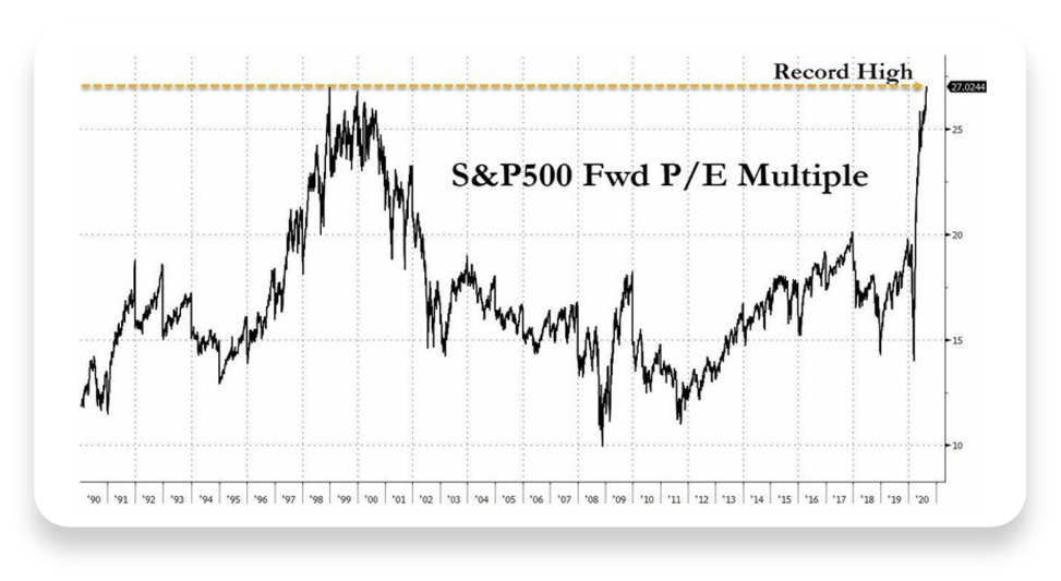
Given that the S&P 500 has just breached the all time high from the peak of the dot-com bubble of the early 2000’s the importance of assessing expected returns is more important than ever.

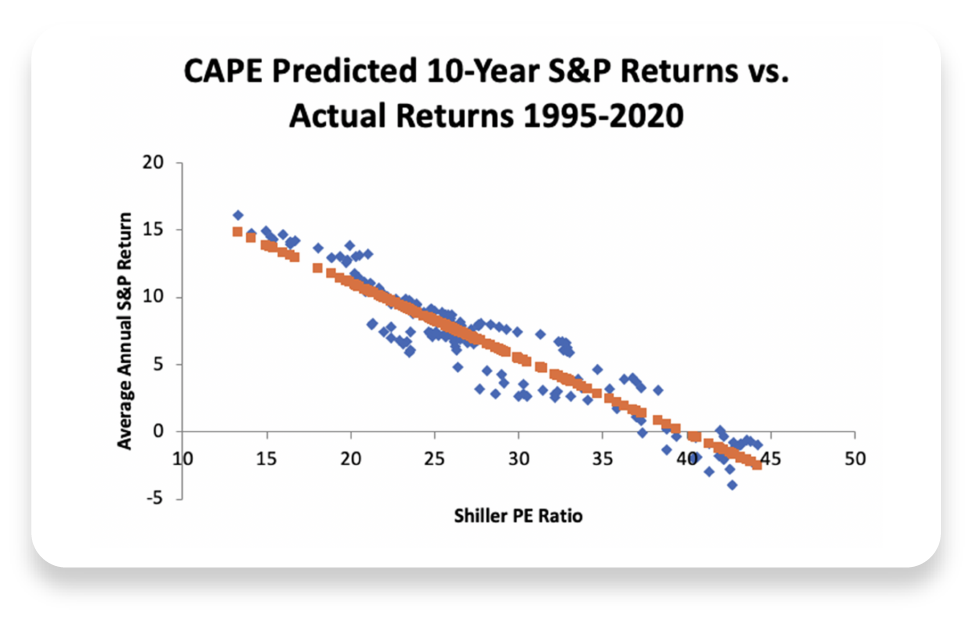
Ownership of a stock is a claim on a very long-term stream of earnings that will accrue to shareholders over time. A stock return consists of the risk-free return and a risk premium, the latter being the amount of extra expected return that is needed to incentivise risk-averse investors into buying a stock instead of a bond. But as the next chart shows, it is intuitively clear that the higher price one pays for an asset, the lower the prospective returns will be.

So can valuations predict returns?
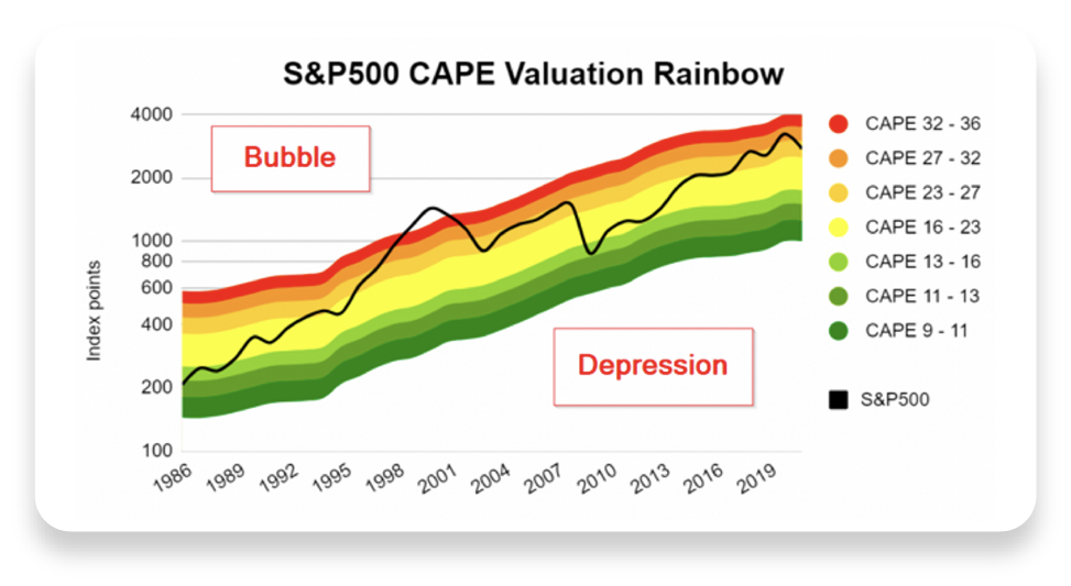
Since 1900, the geometric average US stock returns have been c.10% p.a. But is this a reasonable expectation at all times? According to Shiller, not so; as a result of rising valuations, his most recent (Q1 2020) forecast is for a nominal 10 year annualised return of 4.4%, which is about the same as it was in July 2016. Given a standard deviation of 1.37%, a 10% return would be a 4.1x standard deviation event, which has a 0.26% probability of occurring. Yet, US equities have seen very strong returns on the last 5 years (119.98%), which equates to an annualised 17.08% return, much stronger than the model predicted back in 2016 (and going forward too). The next chart demonstrates that valuations have remained in the upper end of the range, rather than mean-reverting as might have been expected, which explains some of this anomaly. The model cannot account for this phenomenon, as it implicitly provides for valuations to revert to average. The current CAPE reading is around 29x, which implies a long term expected return of around 4.7%, using data going back to 1940, from Professor Michael Finke.

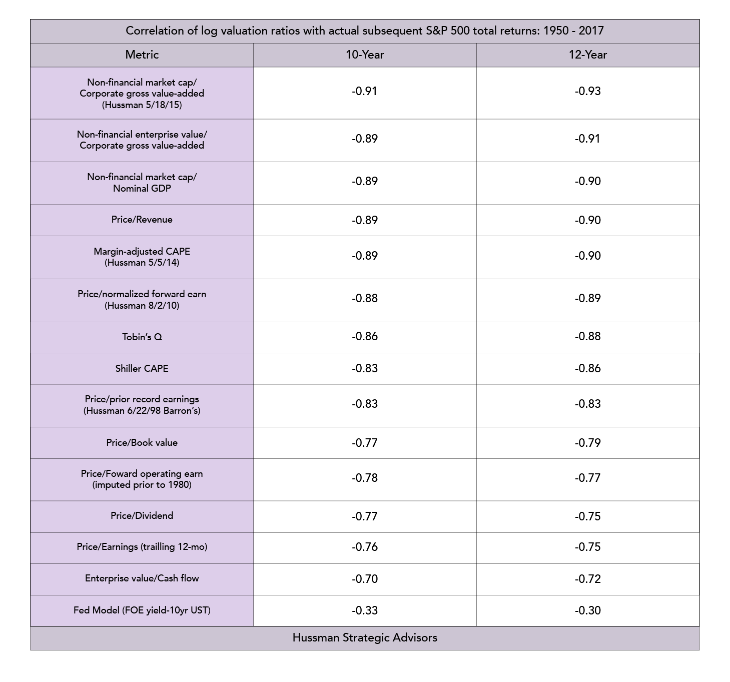
Some have tried to improve on the Shiller CAPE to deal with the profit margin issue raised above. Comparisons of statistical “accuracy” of various alternative methodologies can be seen below (note the very weak relationship between the Fed Model and subsequent actual returns over time, despite its popularity on Wall Street). Most of the other models in this table have a similar correlation with actual realised returns. (The numbers have not significantly changed in the course of the last 3 years).

Why is it so hard to forecast accurately? As active mangers and fundamental analysts frequently discover, at best, economic developments can only be estimated roughly. Although US earnings tend to grow around 6% per annum peak to peak across economic cycles, the earnings growth of internationally oriented companies has over time become more and more decoupled from the economic cycle of their countries of origin, and short- to medium-term earnings growth correlates only very weakly with stock market developments. Unforeseeable developments such as terrorist attacks, oil price shocks or central bank statements, and the resultant market sentiment have a much greater impact on capital market developments in the short to medium term than calculable fundamental data. Robert Shiller could not possibly have foreseen the extent to which Central Banks would back-stop asset prices for example. This meant that investors welcomed the ultra-low interest rates that CB’s ushered in, without asking whether these very same low rates might be a sign that earnings would also be very low.
Creating Estimated Rates of Return (ERR’s) and thus return projections are an extremely imprecise science. Simply taking the average of predictions may well turn out to be as good as any model results, for as we know, the outputs of a model are only as good as the inputs and thus some (maybe a large) margin of error is to be expected. Looking at the table above, it appears that most methodologies yield similar results in terms of accuracy (i.e. correlation). But the map (CAPE) is not the terrain, so there could be a huge variation in asset performance over the 10 years, even if the end result is (more or less) what was predicted.
In similar fashion, a weather forecast can be broadly right, even if one occasionally gets soaked in August. We have learned from experience that weather forecasters rarely get it completely wrong, (which may explain why we enjoy it so much when they do), so, it would be wise to recognise the limitations of CAPE and other models, to avoid a false sense of confidence in investors’ minds; focus less on the absolute return numbers and more on CAPE as a guide rather than a firm indicator of the future- the same applies to any other long-term forecasting model, as over-reliance on any one valuation input is likely to lead to disappointment; in addition, the long-term prognosis is highly path dependent for investors. For example, a 4.4% annualised 10-year return can be achieved via 10 years of +4.4%, or by a 25% drop followed by an 8.3% annual return for 9 years, or literally any other combination of performance numbers. The former may be disappointing, but the latter unacceptable. It is here that the CAPE and other models come into their own, by giving investors a sense of the risk (or likelihood) of very poor returns. If the range of potential returns is too wide, it may be prudent to narrow it, by taking on less (equity) risk.
[1] Consider a cyclical firm with earnings of £2 and a share price of £20, giving it a price to earnings ratio of 10 (20/2 = 10). The problem comes at cycle turning points (I.e. the end of recessions or the end of booms). At the low point, earnings may be only £1 and a price of £10, giving it the same p/e of 10, whilst at the top, earnings may be £4 (price £20) for a p/e ratio of 5. The former may well in fact be cheap (and in the latter case expensive) despite the raw numbers indicating otherwise, due to the fact that earnings are about to grow/decline sharply, giving a misleading impression of the valuation of the firm on a raw p/e basis alone. In sum, p/e’s look worst (most expensive) when earnings have been crushed by recession and best when earnings are flattered by a boom, creating the potential for an investor to buy high and sell low using this naïve valuation model.
Disclaimer
We do not accept any liability for any loss or damage which is incurred from you acting or not acting as a result of reading any of our publications. You acknowledge that you use the information we provide at your own risk.
Our publications do not offer investment advice and nothing in them should be construed as investment advice. Our publications provide information and education for financial advisers who have the relevant expertise to make investment decisions without advice and is not intended for individual investors.
The information we publish has been obtained from or is based on sources that we believe to be accurate and complete. Where the information consists of pricing or performance data, the data contained therein has been obtained from company reports, financial reporting services, periodicals, and other sources believed reliable. Although reasonable care has been taken, we cannot guarantee the accuracy or completeness of any information we publish. Any opinions that we publish may be wrong and may change at any time. You should always carry out your own independent verification of facts and data before making any investment decisions.
The price of shares and investments and the income derived from them can go down as well as up, and investors may not get back the amount they invested.
Past performance is not necessarily a guide to future performance.


